
The main objective of the article is how the world of finance was changed by scientific research throughout the last century, including different hypotheses on the distribution of stocks’ returns starting from normal distribution to Brownian motion; talk about how Brownian motion influences the Heston model.
The world of finance has changed dramatically over the last century, and much of that change has been driven by scientific research. Physics and statistics have had a significant impact on how economists and investors understand financial markets. In this article, we looked at how these two fields influenced the development of financial models, with a particular emphasis on the hypothesis of stock return distributions, the Brownian motion, and the Heston model.
The hypothesis of stock return distributions is one of the most crucial ideas in financial modeling. According to this hypothesis, stock returns have a predetermined probability distribution, which enables economists and investors to forecast future returns. The normal distribution has traditionally been used to estimate stock returns, however this approach has been criticized for its inability to account for extreme market events, such as stock market crashes, into consideration. As a result, in order to better model stock returns, economists and investors have turned to alternative distributions like the power-law distribution i.e., power law distributions with no characteristic scale of phenomena used primarily in physical or social domains such as earthquake magnitudes and war deaths.
Physics - What is a Brownian motion?
It is the incessant and disordered motion of very small particles suspended in water or gas. This was discovered by the Scottish botanist Robert Brown, who in 1827 observed with the microscope pollen particles suspended in water whose rectilinear motion suffered sudden deviations in different directions. The studies then made to explain the phenomenon showed that liquids and gases are made up of molecules in continuous motion and laid the theoretical premises to prove the existence of atoms. In fact, liquid or gas, even if they appear stationary, are sets of molecules in continuous agitation, which thus affect the particle that is immersed in it on all sides. Normally the shocks coming from one direction are compensated by those coming from the opposite direction and the visual effect is of complete immobility. Sometimes, however, the balance is broken, and the molecule is pushed in a random direction. The motion of the suspended particles thus shows that the individual molecules that make up the liquid or gas also move.
Several decades later, in 1900, Louis Bachelier built the foundation of mathematical finance by integrating Brownian motion with the fluctuation in the price of a stock. He postulated that two ideas should be considered when exploring the future value of an asset.
How a collection of anterior events influences the asset.
How the probability of unknown future events could affect the stock price.
For example, the C.E.O of Apple just got replaced yesterday; that is an anterior event that could influence the future price of an Apple stock. On the other hand, if a power outage occurs tomorrow in one of Apple’s factories and halts production, that is an unknown future event that might affect the price of the stock and falls into the second category.
It is said that the fluctuation in the price of a stock attributed to the latter follows Brownian motion as it is seemingly unpredictable and random. Bachelier only focused on the second idea since the anterior events were not meaningful because Bachelier defined the mathematical expectation for an asset to rise or fall to be zero since the market consists of a pool of people that trade with opposite beliefs on the future value of an asset. For example, suppose a person is buying a call option for an asset, they hence believe that its price will rise. The person on the other side of the option believes it will fall otherwise they would not be selling the option. They are both aware of past events that can influence the asset and have contradictory beliefs on how it will perform, meaning the mathematical expectation of the change in value of the underlying asset is neither positive nor negative. The market is therefore said to be fair. Louis Bachelier applying the concept of Brownian motion to asset price behavior, led to Brownian motion becoming one of the most important fundamentals of modern quantitative finance. Combining his assumptions with the central limit theorem, he also deduces that the random behavior of prices can be said to be represented by a normal distribution (Gaussian distribution).
This led to the development of the Random Walk Hypothesis or Random Walk Theory, as it is known today in modern finance. Random walking is a statistical phenomenon in which stock prices move randomly. When the temporal step of a random walk is made infinitesimally small, the random walk becomes a Brownian motion.
Standard Brownian Motion
In the context of financial stochastic processes, Brownian motion is also described as the Wiener process which is a continuous stochastic process with normally distributed increments. Using Wiener process notation, a continuous-time asset price model can be expressed as:

where dS is the change in the price of the asset in continuous time dt. dX is the random variable of the normal distribution (N (0, 1) or Wiener process). σ is assumed as constant and represents price volatility considering unexpected changes that can result from external effects. Together they represent the deterministic return within the time interval with μ representing the growth rate of the asset price or the "drift". When the market is modeled with a standard Brownian motion, the probability distribution function of the future price is a normal distribution.
Properties of a Brownian motion:
Continuity: Brownian motion is the continuous time limit of random discrete-time walking. It therefore has no discontinuity and is everywhere non-differential.
Finite: Time increments are scaled with the square root of time steps such that Brownian motion is finite and always nonzero.
Normality: Brownian motion is normally distributed with mean standard deviation zero and non-zero.
Martingale and Markov properties: The Martingale property states that the conditional expectation of the future value of a stochastic process depends on the current value, given information about previous events. The Markov property focuses instead on the "memoryless" theory according to which the expected future value of a stochastic process does not depend on any past value except the current value. Brownian motion follows both properties.
Random walk
Symmetric random walking can be defined as

where i ∈ Z, which means that variable X has the same probability of increasing or decreasing by 1 at each time step. Now, suppose we speed up this process by taking smaller and smaller steps in smaller and smaller time intervals. If we now go to the limit in the right way, what we get is Brownian motion. Therefore
X(t) = δ x (X1 + .... + X [t/δ t])
Where, Xi = +1, if the i-th step is on the right and Xi = −1, if the i-th step is on the left E [t/δ t] is the largest integer less than or equal to t/δ t. A stochastic process {X(t), t ≥ 0} is called Brownian motion if:

When σ = 1, the process is called standard Brownian motion. Every Brownian motion can be converted in the standard process leaving B(t) = X(t)/σ for standard Brownian motion.
Hitting Time
The first time the Brownian motion hits a is called hitting time.
To show that P {Ta < ∞} = 1 and E(Ta) = ∞ for a 6= 0, consider, X(t) Normal(0,t)
Let, Ta =First time the Brownian motion process hits a. When a > 0, we will compute P {Ta ≤ T} by considering P{X(t) ≥ a} and conditioning on whether or not Ta ≤ t.
So,
P{X(t) ≥ a} = P{X(t) ≥ a|Ta ≤ t} P {Ta ≤ T}
+P{X(t) ≥ a|Ta ≥ t} P {Ta ≥ T}
But, P{X(t) ≥ a|Ta t}=12
By continuity, the process value cannot be greater than a without having yet hit a. So,
P{X(t) ≥ a|Ta ≥ t} = 0
Thus,

For a < 0, the distribution of Ta is by symmetry, the same as that of T−a Thus,


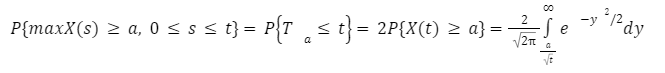
Maximum Time: It is the maximum value the process attains in [0,t]. Its distribution is obtained as follows: For a > 0
To obtain the joint density function of X(t1), X(t2),.....X(tn) for t1 < .....,< tn note first the set of equalities
X(t1) = x1
X(t2) = x2
.
.
.
X(tn) = xn
is equivalent to
X(t1) = x1 X(t2) − X(t1) = x2 − x1 .
.
.
X(tn) − X(tn−1 = xn − xn−1
However, by the independent increment assumption it follows that X(t1),X(t2)− X(t1),......,X(tn) − X(tn−1), are independent and by stationary increment assumption, X(tk)−X(tk−1) is normal with mean 0 and variance tk −tk−1. Hence, the joint density of X(t1),....,X(tn) is given by

From this equation, we can compute in principle any desired probabilities. For instance, suppose we require the conditional distribution of X(s) given that X(t) = B where s < t. The conditional density is

Where, K1,K2 and K3 do not depend on x. Hence, we see from the preceding that the conditional distribution of X(s) given that X(t) = B is, for s < t, normal with mean and variance given by

Distribution of Ta. Suppose a > 0. Since P (Bt = a) = 0 We have
P(Ta ≤ t) = P(Ta ≤ t,Bt > a) + P(Ta ≤ t,Bt < a) (1)
Now any path that starts at 0 and ends above a > 0 must cross a, so
P (Ta ≤ t,Bt > a) = P(Bt > a) (2)
To handle the second term in the equation (1), we note that
(i) The strong Markov property implies that B (Ta + t) − B(t) = B(Ta + t) − a is a Brownian motion independent of Br, r ≤ Ta and
(ii) The normal distribution is symmetric about 0, so
P (Ta ≤ t,Bt < a) = P(Ta ≤ t,Bt > a) (3)
This is called the reflection principle, since it was obtained by arguing that a path that started at 0 and ended above a had the same probability as the one obtained by reflecting the path Bt,t ≥ Ta is a mirror located at level a.
Combining equations (1), (2) and (3), we have,


Proof: If Bs = a > 0, then symmetry implies that the probability of at least one zero in (s,t) is P(Ta ≤ t−s). Breaking things down according to the value of Bs, which has a normal (0,s) distribution, and using the Markov property, it follows that the probability of interest is

(7)
Interchanging the order of integration, we have
The inside integral part can be evaluated as So, equation (7) becomes
Changing variables r = sv^2, dr = 2svdv produces

By considering a right triangle with sides s, t − s and t one can see that when the tangent is p(t − s)/s and cosine is ps/t. At this point we have shown
that the probability of at least one zero in (s,t) is (2/π)arccos(ps/t). To get the result given, recall arcsin(x) = (π/2) − arccos(x) when 0 ≤ x ≤ 1.
Let Lt = max {s < t: Bs = 0} So,

(8)
Recalling that the derivative of arcsin(x) is 1/sqrt(1 − x2), we see that Lt has density function

In view of the definition of Lt as the LAST ZERO before time t, it is somewhat surprising that the density function of Lt (i) is symmetric about t/2 and (ii) tends to ∞ as s→0. In a different direction, we also find it remarkable that P (Lt > 0) = 1. To see why this is surprising note that if we change our previous definition of the hitting time of 0 to T0+ = min {s > 0 : Bs = 0} then this implies that for all t > 0 we have P(T0+ ≤ t) = P(Lt > 0) = 1 and hence
P (T0+ = 0) = 1 (10)
Since, T0+ is defined to be the minimum over all strictly positive times, equation (4) implies that there is a sequence of times sn → 0 at which B(sn) = 0. Using this observation with strong Markov property, we see that every time Brownian motion returns to 0 it will immediately have infinitely 0’s!
Brownian Motion for Financial Mathematics
The mathematical theory of Brownian motion has been applied in contexts ranging far beyond the movement of particles in fluids. Until recently, stock market researchers have confronted the same problem. While they can chart the path of the market on a minute-by-minute basis it is very hard for them to observe who buys, who sells and how demand and supply affects price movements. There exist many interesting theories about how the behavior of different investors makes the prices move, but there is no empirical evidence to support the critical link between the investor decisions and the price dynamics. However, stock markets, the foreign exchange markets, commodity markets and bond markets are all assumed to follow Brownian motion, where assets are changing continually over very small intervals of time and the position, namely the change of state on the assets, is being altered by random amounts. More importantly, the mathematical models used to describe Brownian motion are the fundamental tools on which all financial asset pricing and derivatives pricing models are based.
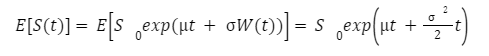
Geometric Brownian motion

dS is the change in the price of the asset in continuous time dt. dX is the random variable of the normal distribution (N (0, 1) or Wiener process). σ is assumed as constant and represents price volatility considering unexpected changes that can result from external effects. μdt together represent the deterministic return within the time interval with μ representing the growth rate of the asset's price or "drift". When the market is modeled with geometric Brownian motion, the probability distribution function of the future price is a log-normal distribution.
Basic Properties:
Return Values Sti+1/Sti are independent for

Simply an exponentiated Brownian Motion => only positive values
Mean: (using moment generating function)
Variance:


Simulation of random walks for stock prices
In quantitative finance, a Random Walk can be programmatically simulated through coding languages. This is essential because these simulations can be used to represent potential future prices of assets and securities and solve problems such as derivatives pricing and portfolio risk assessment.
A very popular mathematical technique to do this is through Monte Carlo simulations. In options pricing, the Monte Carlo simulation method is used to generate multiple random walks representing the price movements of the underlying, each with a simulated payoff associated with the option. These payoffs are discounted to the current value and the average of these discounted values is set as the option price. Similarly, it can be used for pricing other derivatives, but the Monte Carlo simulation method is most used in portfolio and risk management.
For example, consider Microsoft stocks that have a current price of $258.65 with a growth trend of 55.2% and volatility of 35.92%.
A chart of daily returns represented as a random normal distribution is:

The preceding figure represents the simulated price path based on geometric Brownian motion for the Microsoft stock price. Similarly, a graph of 10 simulations of this type would look like this:

So, we can see that with only 10 simulations, prices range from $100 to over $600. We can increase the number of simulations to expand the dataset for analysis and use the results for derivatives pricing and many other financial applications.
HESTON MODEL
The Brownian motion has also played a key role in the development of the Heston model. It is a widely used financial model that was first introduced by Steven Heston in 1993, it is not the only study devoted to the valuation of financial derivatives under such assumptions, but it has become the standard against which other models proposed in the literature as a natural extension of the famous formula of Black, Scholes (1973), widely used in the field of financial applications, have been evaluated over time. The Heston model assumes that stock prices and volatility are correlated, and it describes volatility as a stochastic process that follows a geometric Brownian motion.
In comparison to other financial models, the Heston model has several advantages, including its ability to more correctly describe the dynamics of financial markets and its ability to accurately price financial options, such as call and put options.
It is crucial to take into account the idea of stochastic calculus in order to comprehend how the Brownian Motion affects the Heston model. Stochastic calculus is a field of mathematics that deals with the integration of random processes, and it has become an essential tool for financial modeling. In the Heston model, stochastic calculus is used to describe the correlation between stock prices and volatility, and to model the random fluctuations of both variables.
Risk analysis, portfolio management, and option pricing are just a few of the financial areas where the Heston model has been extensively employed. However, the model has also been criticized for relying too heavily on the normal distribution of stock returns, which isn't necessarily a reliable indicator of market behavior. The Heston model may also be challenging to use, requiring sophisticated mathematical methods and advanced techniques and significant computational resources.
The Heston model continues to be an important resource for economists and investors all around the world, despite its limitations. It has become an important instrument in risk analysis and portfolio management due to its capacity to accurately characterize the dynamics of financial markets and price financial options. Moreover, the model has also sparked a variety of studies in the domains of statistics, physics, and finance and is still a hot topic for both academics and industry professionals. For example, in a 2014 paper titled "A Review of the Heston Model and Its Variants", professor Dilip B. Madan and his co-authors provide a comprehensive review of the Heston model and its various extensions and modifications. The authors note that while the Heston model has been criticized for its reliance on the normal distribution, it remains a useful tool for pricing options and for analyzing volatility in financial markets.
It is generally described by the following equations:

Where k represents the rate of reversion to , which is the long term variance.
In addition to the Heston model, there are many other financial models that have been developed over the past century. These models have been inspired by a wide range of scientific disciplines, including physics, mathematics, and statistics.
For example, the Black-Scholes model, which is used to price options, was inspired by the heat equation in physics. The CAPM model, which is used to estimate the expected return on an asset, was developed by economist William Sharpe and is based on the concept of risk-return tradeoff.
To sum up, over the last century, the fields of physics and statistics have had a significant impact on the development of financial models. Stock return distributions have been extensively studied, and researchers have looked to alternative distributions, such as the power-law distribution, to better model extreme market events. The Brownian motion has been used to describe the random fluctuations of stock prices and has played an important role in financial modeling. The Brownian motion-based Heston model has become a widely used financial model that has been applied in many different areas of finance.

コメント